Propagation of uncertainty calculates the effects of the uncertainty in system inputs on the system outputs. This information is critical when quantifying confidence in a system's outputs.
Propagation of uncertainty helps determine whether system outputs will meet requirements given the anticipated variation in inputs. This makes it possible to estimate the probabilities of outcomes, to cost effectively determine required tolerances, and to predict more failures before they happen.
SmartUQ delivers advanced stochastic mathematics in an easy-to-use tool and features two ways of calculating propagation of uncertainty, emulator based and generalized Polynomial Chaos expansion (gPCE).
Propagation of uncertainty calculates the uncertainty in a system's outputs based on the uncertainty associated with each of the system's inputs. All models, predictions, and measurements have uncertainty associated with them. Uncertainty in various inputs, such as initial conditions, environmental parameters, and measurement error can all effect the outcome of a simulation or test in unexpected ways.
Knowing the source and scale of uncertainty in simulation and testing results is critically important when determining if a design or decision will be successful. Thus, propagation of uncertainty is a vital tool when providing a solid basis for high-consequence decisions.
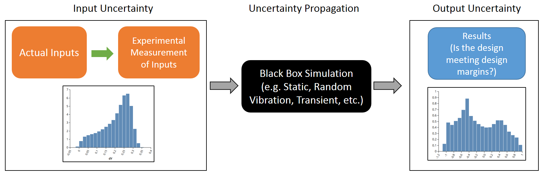 Figure 1: Propagation of Uncertainty Information Flow
Historically, propagation of uncertainty results were calculated by running system inputs using large DOEs, such as Monte Carlo methods, and observing the output behavior. Unfortunately, for large-scale and high dimensional problems, the required DOE sizes are very large and it becomes prohibitively expensive and slow to calculate the propagation of uncertainty. emulator/surrogate model based propagation of uncertainty calculation has become a popular solution due to the increase in speed over more sampling intensive methods. But the use of emulators is often limited to smaller problems as building emulators with large and complicated data sets is computationally difficult.
Now, with the use of SmartUQ's breakthrough technologies, emulator based propagation of uncertainty for large scale problems is only a few clicks away. Our intuitive tools allow you to quickly take a previously constructed emulator and define uncertain inputs using either probability distributions or existing input parameter sets such as those from anticipated system operating conditions or recorded tests.
Example
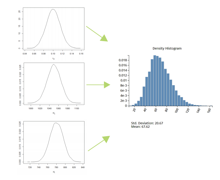
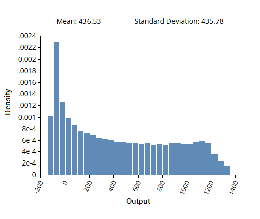 Figure 2: Emulator Based Propagation of Uncertainty
In this example, an emulator was built and used to calculate the propagation of uncertainty for a simulation data set consisting of three input variables and a single output variable. The input variables were assigned probability distributions based on their expected uncertainty. The calculated density distribution for the output, given the assigned input distributions, is shown above.
SmartUQ features an easy to use Generalized Polynomial Chaos Expansion (gPCE) tool. gPCE is an applied mathematics technique for estimating the behavior of a system using a series of multivariate polynomials. The system to be evaluated is sampled using a sparse grid DOE and then gPCE is used to approximate the functional association between the stochastic output and each of its random inputs. This approximation is then used to calculate uncertainty propagation and sensitivity analysis results. gPCE is a highly efficient technique both in the low number of points required in the sparse grid DOEs and in the speed of calculation of the results.
For an output, the gPCE can be written as a series of multivariate polynomials. The multivariate polynomials are themselves comprised of one-dimensional polynomials. Each one-dimensional polynomial provides an optimal basis for different continuous probability distribution types. The optimality of each basis comes from its orthogonality with respect to the probability density function of the continuous distribution.
Example
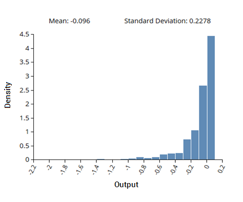 Figure 3: Generalized Polynomial Chaos Expansion for Propagation of Uncertainty
In this example, gPCE based methods were used to calculate the propagation of uncertainty on a data set consisting of five input variables and a single output variable. The input variable probability distributions were predicted based on their expected uncertainty and this was used to generate the sparse grid DOE. The system was then evaluated using the DOE and the resulting outputs were used in the gPCE analysis. The calculated density distribution for the output, given the input probability distributions, is shown above.